


From what we can tell, Murphy’s Law (which in its most famous form states: “If anything can go wrong, it will”) was supposedly first coined...
From what we can tell, Murphy’s Law (which in its most famous form states: “If anything can go wrong, it will”) was supposedly first coined at Edwards Air Force Base in the United States around 1949. While many seem to claim credit for the concept, it appears that it was named after Capt. Edward A. Murphy, an engineer working on a project for the Air Force to see how much sudden deceleration a pilot could withstand in a crash. As the story goes, one day, after finding that a piece of equipment was wired incorrectly, Captain Murphy cursed the technician responsible and said, “If there is any way to do it wrong, he’ll find it.” The contractor’s project manager kept a list of “laws” and upon hearing this statement added this to his list, which he simply called Murphy’s Law. Sometime afterward, an Air Force doctor, Dr. John Paul Stapp, who participated in the deceleration project, rode a sled on a track to a stop at rate of over 40 Gs (or about 392 meters per second squared). When he gave a press conference, he noted that their good safety record on the project was due to a firm belief in Murphy’s Law and in the necessity to try to circumvent it. The rest, as they say, is history.
And so it is with analytics and text analytics in particular. Regardless of the amount of planning or forethought put into a project, something always goes wrong. Sometimes it’s something small, perhaps an oversight; other times it could be as large as making some incorrect assumptions and having to start from the beginning. No matter, the objective isn’t to remove all possibilities of things going wrong, but rather simply to be prepared for them.
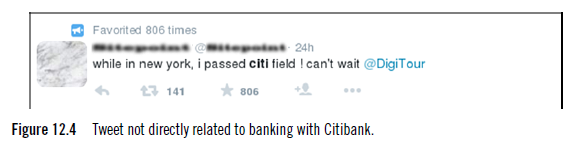
While Figure 12.1 represents our view of an iterative approach to an analytic analysis, it’s impossible to diagram every step of a process, especially as we make subtle changes to tools or search terms. However, we believe this represents a respectable view of the process and therefore the points where things could go wrong.
Previously, we described the process as the five Ws—Who, What, Where, When, and Why. Having a crisp description of what we are looking for may seem obvious to most (step 1 in Figure 12.1), but sometimes we can be stubborn. Often we don’t think that the question we are asking is the right one, or perhaps we need to modify it. We see this later in the examples, but for now, we express the first step as “defining the problem” or perhaps simply “posing a question to be answered.” For example, “What do teenagers think of the latest movie trailer for an upcoming new release?” or “How is our brand perceived in the European marketplace?”
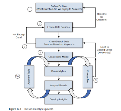
Obviously, when we know the question we want to answer, our next step (labeled step 2 in Figure 12.1) is to find the data that will help us uncover that answer. This shouldn’t be a long, tedious step, but it’s important, if nothing else, as a litmus test regarding the analysis. By this, we mean that if we check for data around this topic, and we find sufficient evidence that is enough to produce a meaningful result, we can (and should) proceed for an analysis. How do we know that we have enough data? The real answer is: We don’t. At least not until we’ve done an analysis to see if there is a sufficient number of results to warrant a conclusion. But again, a quick scan of social media sites or search on Twitter can give us a gut feel that we do or do not have enough material to work with. If we don’t, perhaps, as the diagram shows, we need to modify the question we are trying to answer. When we believe there is sufficient data for our analysis, we then need to go out and collect as much as we can from a variety of social media venues (step 3). Although we may ensure that we include a particular set of sites, if we’re going to use a search engine or a message board aggregator (we tend to use Boardreader because it’s tightly integrated with IBM’s Social Media Analytics [SMA] product) but we can’t be quite sure what sites or content will be returned. This isn’t a bad thing; the problem is that there are so many social sites that could possibly contain content relevant to our question. The work done in step 2 was just a cursory check; now we put in a set of keywords and ask for all the matches.
Developing a data model (step 4) is a process or method that we use to organize data elements and standardize how the individual data elements relate to each other. This step is important because we want to run a computer program over the data; we need a way to tell the computer which words or themes are important and if certain words relate to the topic we are exploring. For example, if we were looking at job titles or descriptions, the word architect may come up. If we were specifically interested in the computer field and information technology professionals, we would want to qualify the word architect with some technical words such as network so that we could find network architect or terms such as system or computer to uncover discussion around system architect or computer architect. This is what a data model does for us: it defines our “universe” and creates relationships between words and phrases so that we can make sense of the data during our analysis.
In the analysis of our data, it’s handy to have several tools available at our disposal to gain a different perspective on discussions taking place around the topic. We like to call this “our bag of tricks.” In some cases, it may make sense to look at a word cloud of conversation, and in others, it may make sense to watch a word cloud evolve over time (so computing a time series word cloud may make sense). When we talk about step 5a, augmenting the tools, that’s really about configuring them to perform at peak for a particular task. For example, thinking about a word cloud again, if we took a large amount of data around computer professionals, say the IT architect example from the previous step, and built a word cloud, no doubt the largest word in the cloud would be architect. (Remember, in word clouds, the more frequent a word is used, the larger it becomes in relation to the other words.) So here, we might create our initial cloud, see that architect is overwhelming the cloud, and simply change the configuration to eliminate that word. Think about it: we know the data collected has to do with IT architects, so why do we need to show it in our cloud? By eliminating it, we allow other words to stand out and perhaps reveal some insights.
This analysis is also about tool usage. Some tools may do a great job at determining sentiment, whereas others may do a better job at breaking down text into grammatical form (noun, verb, adjective, and so on) that enable us to better understand the meanings and use of various words or phrases. As we said, it is difficult to enumerate each and every step to take on an analytical journey. It is very much an iterative approach (perhaps we should call it “exploratory analysis”) as there is no prescribed way of doing things. But with that said, let’s take a look at some of these steps and see where things can (and undoubtedly, will) go wrong.
In 2012, there was a scandal involving Chinese factory workers and the conditions under which they were expected to work. Several US-based firms were “called out” in the press for using these companies in the production of their products. The question we were trying to answer was: “Is IBM being associated with potential “bad press” in any of the social media venues?” And if so, where? Also, what is the perception of IBM in relation to its competitors?
A quick manual survey of various wiki and blog sites showed there was indeed conversation happening around this particular event and factory. With that in mind, our plan was to mine the social media space for any occurrence of the particular factory which included mentions of IBM and then build a more comprehensive model to understand the conversations. This model would consist of key terminologies that may (or may not) reflect the public’s perception of the factory worker’s concerns. Later revisions would then take this analysis and segment it by various competitors to see how IBM was viewed amongst its competitors.
Upon collecting all of the available data and subjecting it to our analytic model, we began to build a set of insights. One of the first metrics we produced was a count of the number of mentions This is the number of times various companies, including IBM, were mentioned in all of the social media content that we were able to collect. We also began to summarize the locations where these conversations were taking place. This is an important piece of information not only for obtaining unsolicited opinions but also for marketing and relationship building. There may be a time when we may want to participate in the conversation.
We plotted this information on a bar graph using two bars for each company (Figure 12.2). The first bar in each grouping (on the left) shows data that we first collected (labeled “no city specified”). At first glance, this looks like a major problem for IBM. The graph is showing that there are a large number of references to IBM in the context of this company and the working conditions in various Chinese factories.
A closer look at our results showed that this particular company operated many different factories across China and Asia in general. Our first interpretation was that people were associating IBM with this event. However, we came to realize that the poor working conditions were limited to a factory in a single city. Once we realized that, we limited our model to that particular city and then any mentions of IBM and its competitors. The result was the second bar (the one on the right in each grouping) in Figure 12.2 (labeled “in the context of a city”). As it turned out, there was no association of IBM and the factory in question.

The reason we received these types of results wasn’t so much that our data was flawed; but for this particular analysis, it just wasn’t scoped properly. The moral of this story: double-check your findings early and often. Had we continued to build out a full analysis based on this data, it would have been like attempting to ask the crowd at a baseball game what they thought about a movie premiere; that is, data about a topic from a completely unrelated source.
What makes social media analytics, or any kind of text analytics for the matter, difficult is that most of the data we’re looking to analyze is unstructured or maybe better said—not consistent. The problem is that we humans have different ways of saying the same thing. What we say or how we say it may make sense to us, but often it is unclear to others. The English language is funny; many people claim it’s one of the hardest languages to master. Consider the case of words that are classified as homonyms (words that have the same spelling and pronunciation but have different meanings).
We’ve seen a number of these issues when we start a new analysis. Let’s take our analysis of financial institutions as an example. We were looking at how the public views various banking establishments and what their views on savings were.
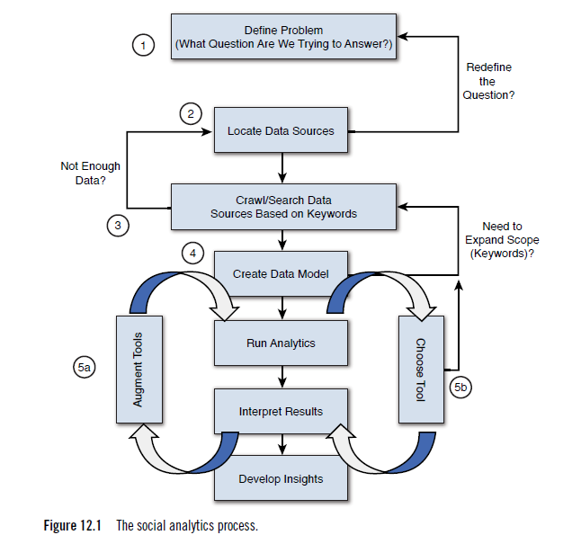
One of the banks we tried to gather social data mining discussion on was Citibank . It has a very active Twitter account, and a quick search for viable information showed a fairly high level of activity. In our collection of data, we uncovered other banks that were also generating a fair amount of social media mentions. In Table 12.1, these banks are labeled Bank-1, Bank-2, and Bank-3.
What’s interesting about this bank is that it has a number of Twitter handles for specific geographies—for example, @citibankau (Australia), @citibankIN (Citibank Indonesia), and @citibankeurope. Consequently, our assumption was that the data we were collecting was for US banks (which was the scope of our experiment). What we forgot about was the fact that Citibank also sponsors a baseball stadium for the New York Mets in New York City. So as we pulled information from Twitter, we used the search term citi (as well as a few others like @citibank, and so on). When we did the first pass at our analysis, we had some preliminary statistics, as shown in Table 12.1.
One of the topics we included in our analysis was the public’s perception of certificate of deposit (CD) rates and offerings from various banks. In this instance, when we were gathering data, we included reference to home (mortgage) loans, refinancing, lines of credit, and CDs.
Unfortunately, the term CD is another homonym:
CD, as in certificate of deposit
CD, as in compact disc
In Table 12.1, notice the large amount of discussion around bank products (CDs were grouped under Products). We had to rework our data model to qualify the word CD with the word bank. This showed a bit of improvement, and things got a little better, but a quick look at Figure 12.3 shows the kinds of tweets we were still collecting. Clearly, we still had more work to do. The good thing was that the incorrect (and the correct) use of the word CD was applied to all the banks. That just means we had less confidence in discussion around that topic.
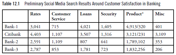
 Our bigger problem was with the references to baseball around Citibank. The odd part of this was the more than 3,000 uncategorized statements for Citibank. We expected a number of comments or tweets to be uncategorizable, but this number was off by a factor of 100× compared to the others. A closer inspection showed a large number of references to baseball and sports. This result wasn’t too unusual because we knew that many large corporations (banks included) sponsor sporting events or teams. But then we uncovered tweets such as shown in Figure 12.4.
 While this was potentially an important message if we were looking only at Citibank (and the positive sentiment surrounding its backing of a baseball team), in this case, such tweets were not at all relevant to our experiment.
We had two choices at this point. Referring back to Figure 12.1, we could:
■ Rework the question we were trying to answer (step 1)
■ Look to eliminate discussion about citi field (step 4)
Understanding That Sometimes Less Is More
Because we are programmatically pulling data into our analytics software, we sometimes have to be careful not only about the mislabeling of data, but in this case the duplication of data.
In one case, we were looking at a number of issues across the information technology industry, and we wanted to see where IBM ranked in the discussion along with several leaders in this space. When we pulled our data and started to group the number of mentions by company, we produced a graph that looked something like Figure 12.5.

Upon careful inspection, we discovered that many of the items in our data collection were duplicated entries. For example, the mentions around apple numbered around 347 specific references; Microsoft, about 95; and so on. Our analytics just didn’t look right as we continued our analysis, and eventually, we realized that many of the entries in the sample were duplicates.
the Web URL is: http://thecrux.com/dyncontent/psibookmf_next-big-financialcrisis-coming-soon/?cid=MKT015071&eid=MKT035893&snaid=&step=start
So if we pull data from this site (assuming we used the keywords hedgefund and crisis), it would be mapped to that URL as the source. But say another web page linked to it and used this URL: http://thecrux.com/dyncontent/psibookmf_next-big-financialcrisis-coming-soon/?cid=MKT015071&eid=MKT035893 In this case, both would return the same exact content, but because the URLs are different (notice the missing &snaid=&step=start at the end of the second URL), they appear to come from different sites.
We implemented a data duplication algorithm in our process, and as a result, the number of unique mentions of apple went from 347 to about 81 (just as Microsoft went from 95 to 34). The number of items for the other entities also decreased significantly, forcing us to reevaluate our data sources and keywords to search for more data. Note that our process of eliminating data is different from data deduplication. The concept behind data deduplication is essentially to save on storage (and the repeated storing of the same object). Data deduplication (sometimes called single-instance storage) is a technique that is often used to reduce storage needs by eliminating redundant data. In many cases, only a single unique instance of an item is retained in an archive; any redundant use of the same item is simply replaced with a pointer to the single copy.
Think of email as an example. How many times has someone sent a large file to a large distribution list, only to have numerous people “reply with history” and forward a copy of the large file. In the end, everyone’s email inbox gets flooded with numerous copies of the same large file. By using a data deduplication technique, only one instance of that large file would be stored, and all subsequent uses would simply point back to the original. In our case, we didn’t want that. If the item of text (or discussion) was the same, we simply wanted to remove the redundant entry from our analysis. If someone made reference to the URL pointing to the content, that was fine. But if someone cut and pasted the content from one URL to a unique URL, we would eliminate the second source.
Customer Service for xyz company is the worst I’ve ever seen. Most applications will scan over the words used in a set of text and simply add up all the positive words and all the negative words. They then subtract the count of positive words from the count of negative words to produce a score:
Positive Score – Negative Score = Sentiment Score
If that score is positive (that is, there were more positive words than negative), the overall sentiment is said to be positive. If the count of negative words is higher than the count of positive words, the subtraction of the positive word count from the negative will produce a negative number, indicating an overall negative sentiment. In the preceding example, if we were to use this scoring method, we could derive: A count of zero for the positive terms (there were no clearly positive words in the text) A count of one for the negative terms (the word worst) And then using the preceding formula, we would derive an overall sentiment score of:
0 (the positive score) – 1 (the negative score) = –1
So in this case, we would obtain a score of –1, indicating that the text is basically presenting a negative sentiment. There can be many variations on this algorithm, which tends to produce several shades of gray in the answer. For example, in the tweet shown here, the word service could be considered a positive term, although perhaps not as positive as words such as good, fantastic, or excellent. So the system may choose to score that word as slightly positive and assign it a score of +0.25 rather simply considering it as being equal to other words that have a stronger connotation of positive.
As an example, consider these two tweets:
Tweet 1: I thought the movie was decent.
Tweet 2: That was a great movie!!!
With both of those tweets, if we were to use the algorithm described here (simply counting the number of positive and negative words), both of these tweets would have a positive sentiment score of +1.0. Tweet 1 would be positive because the word decent is considered to have a positive connotation, and no negative words are used. In the case of Tweet 2, no negative words are used, and the word great would be viewed as positive, which would generate a score of +1.0.
However, that may not really be representative of the true intent. Tweet 2, while representing a positive sentiment, is less enthusiastic. In this case, it would be good to give the word decent (along with phrases like not bad, passable, or acceptable) scores that differed from words like excellent, thrilling, or stellar.
In our case, we gave the word decent a positive sentiment of +0.25. So it’s considered positive in sentiment, but only one-quarter that of other words, such as great, which would get a full score of +1.0. So in these examples, Tweet 1 would be of positive sentiment with a score of +0.25, and Tweet 2 would have a positive score of +1.0, indicating the greater sense of positive connotation.
This is where our customizations come in (Step 5a in the flowchart from Figure 12.1). We may need to add (or subtract) a number of words from a dictionary based on their use. Consider the commonly used words shown in Table 12.2. How should each word be treated? Should it be treated as implying a positive sentiment? Or should it be treated as connoting a negative sentiment? The choice can seem quite arbitrary, but as long as we’re consistent in our dictionary augmentations, this can add tremendous value to our analytics.
 Most of the time, when we look at microblogging content (Facebook, Twitter, LinkedIn, and so on), we find that most of the content is fairly neutral—that is, neither positive nor negative in score. Think of a Facebook post that says:
Attending a session at #IBMAmplify on the use of Social Media Analytics There may be some interesting information to be gained from this posting, but there is no particular feeling being expressed. We tend to find that a large amount of microblog content is like this (which is fine). One of the issues we run into when doing a sentiment analysis is considering the use of words such as disaster—a word that clearly indicates some kind of negative sentiment. Consider the following LinkedIn update, for example: Spending my day reading about disaster recovery products on the market today.
Using the algorithm we outlined previously, the sentiment score of this post would be computed at a –1.0 (since disaster would be found in the negative dictionary, and there are no other words found in the positive dictionary). However, when the word recovery is used in conjunction with disaster, our sentiment score should be computed as zero (or the expression of no particular feeling) because the phrase disaster recovery really isn’t positive or negative. We’ve seen this situation countless numbers of times, where the negative connotation of the word disaster essentially cancels out the positive sentiment expressed around it.
We also employ a number of IBM commercial products such as IBM’s Social Media Analytics, SPSS, IBM Content Analytics, and various Watson services now available on Bluemix. Many of these tools specialize in a particular facet of the overall process. For example, SMA does an excellent job of deriving sentiment and summarizing data, whereas SPSS allows for a greater flexibility and deeper statistical analysis. What we’ve learned over time is to take the best parts of each of these tools to derive a more complete answer to the question we are trying to answer. We’ve often found ourselves sticking firmly to a specific tool rather than being open to a variety of results.
One of the engagements we worked on was the public’s perception of various home improvement and appliance stores within the United States during this period. Specifically, we were looking at the public’s reaction to updates, news about needed supplies, and the various responses to emergencies from these companies.
In this case, our main source of data was the public microblogs (Facebook and Twitter). Almost immediately the public gravitated toward a number of hashtags, and our first pass was to focus on them as a way to gather data. Our filters included the following (there were many more in the end; this is just a sampling):
#sandy
#sandyhelp
#hurricane
#Hurricanesandy
#Hurricanesandyproblems
#sandyaid
#sandyvolunteer
#NYCSandyNeeds
#HelpStatenIsland
#SandyReports
#frankenstorm
#hoboken
#sandytoday
#hoboken411
#noheat
#nopower
This example raises an important point about both gathering data and promoting trackable events. By using a hashtag, individuals are telling others that the comment they are making or information they are providing is directly related to a specific event. This point is important because it can really help alleviate any problems with data validity. Since it’s already tagged by topic, we can be somewhat assured that it is part of the dataset we might be interested in. So, in establishing your own social network data media campaign, having a unique hashtag makes the job of doing analytics around the campaign that much easier. Please note that if you were to use a common hashtag (say #ff— Follow Friday) because your event happened on a Friday, be prepared to do a lot of data cleansing and filtering, since much of the data will be unrelated to your event. From an analyst’s perspective, you would be increasing the amount of noise in your dataset and drowning out the signal (the relevant information). We always want to keep the signal-to-noise ratio as high as possible, or maybe better said, we have to have data about our topic (the signal) than the other nonrelated issues (the noise).
A number of interesting positive as well as negative statements were made about a number of the organizations. Specifically, they were being criticized for not donating plastic bags for some of the relief efforts or closing stores early before the storms hit (claiming they cared more about their employees than the general population that was “in need”). On the positive side, a number of comments were made on the helpfulness of the employees and the fact that some stores brought in extra inventory (such as generators or pumps) early in anticipation of the storm. Overall, there seemed to be an equal amount of positive and negative sentiment.
What we really wanted to understand, however, was what topics or issues the general public was raising during this catastrophe. Using SMA’s Evolving Topics tool, we were able to look at terms or phrases that were used over the span of time that we were investigating in an attempt to uncover frequently mentioned topics (see Figure 12.6). The Evolving Topics algorithm identifies word phrases that occur multiple times within the same document and also across multiple documents, so our hope was that this would uncover some interesting insights.
 While we appreciate how SMA can do an analysis across its dataset, we were having trouble uncovering the main points of the conversations that were happening. Although we had a significant amount of time invested in the creation of our SMA models, we still weren’t getting the results we needed to answer our question. Looking back to Figure 12.1, we had all of the data we were ever going to get, so it wasn’t a matter of looking for more or different content. It really came down to how we did the analytics and what tools could “tease” those insights out of our data (steps 5a or 5b).
IBM Watson Content Analytics (then called simply IBM Content Analytics, or ICA) is a tool that breaks down content into facets (see an example of an ICA analysis in Figure 12.7). The Content Analytics engine then provides data about the frequency and correlation information for keywords of the specific facets. Facets can be nouns, noun phrases, verbs, adjectives, and so on. What we are showing in Figure 12.7 is from a different analysis, but we wanted to illustrate the power of ICA and its ability to segment text into its grammatical components. From this analysis, we can begin to derive the topics of conversations and the frequency with which they are happening.
Think of what a noun is. It’s the subject of a sentence or a comment. The verbs describe the intensity of the topic or how people are feeling. Exporting our data from SMA and then re-importing into IBM Watson Content Analytics allowed us to create a list of top topics on the minds of people during this event (see Figure 12.8).
This list was exactly what we were looking for: the topics that people were discussing during the storm as they related to various home improvement centers. We were then able to generate increased sets of metrics and insights based on these themes. For example, when the discussion of generators arose, almost 50% of the discussion was around the need and the urgency of the need for them, while 32% complained of out-of-stock issues. This seems to be an interesting (and measurable) metric that store managers may want to have in the future (hopefully, a future catastrophe isn’t as severe).
So while this example might not be a case of something going wrong, it could have been. Things could have gone wrong had we attempted to use just a single tool in our quest to answer the questions posed. Sometimes we need to take a step backward (or perhaps sideways) to make progress forward; such is the life of an analyst.
Through this analysis, we were able to uncover a number of issues raised by consumers about the various home improvement stores in the area. We were able to report that many consumers were actively looking for batteries and generators during the storm; these items were clearly understocked by many of the stores. What was actually an unanticipated finding was a backlash aimed at the employees of some of the stores. It seemed that many of them abandoned the stores as the storms hit, leaving consumers with no place to turn for those batteries or generators. Those comments were teased from the dataset based on the keywords that arose from the evolving topic graph in Figure 12.6.
And so it is with analytics and text analytics in particular. Regardless of the amount of planning or forethought put into a project, something always goes wrong. Sometimes it’s something small, perhaps an oversight; other times it could be as large as making some incorrect assumptions and having to start from the beginning. No matter, the objective isn’t to remove all possibilities of things going wrong, but rather simply to be prepared for them.
Recap: The Social Analytics Process
Up to this point in this book, we have discussed the various steps we need to take on the journey to analyze social media data collection content. We’ve tried to focus on the “what’s possible” rather than the “how to” because tools and data sources are constantly changing and evolving. But more importantly, we’ve tried to take a logical step-by-step discussion of what needs to be done in performing an analysis, from posing a question, to gathering and cleaning data, and then on to doing the analysis. Consider the diagram in Figure 12.1. Many of the steps in this diagram have been discussed in previous posts and should be familiar to you. The thing to consider is that an analysis isn’t a single, well-defined set of steps; it tends to be quite iterative in nature. That is, we try something, perhaps searching for a set of data; if it appears we have the correct data sources, we go on to the next step to collect data points. If we then determine we don’t have enough data or the correct data, we go back and look for new sources rather than continue with faulty information. Over time, as we iterate through the problem, the answers begin to emerge.While Figure 12.1 represents our view of an iterative approach to an analytic analysis, it’s impossible to diagram every step of a process, especially as we make subtle changes to tools or search terms. However, we believe this represents a respectable view of the process and therefore the points where things could go wrong.
Previously, we described the process as the five Ws—Who, What, Where, When, and Why. Having a crisp description of what we are looking for may seem obvious to most (step 1 in Figure 12.1), but sometimes we can be stubborn. Often we don’t think that the question we are asking is the right one, or perhaps we need to modify it. We see this later in the examples, but for now, we express the first step as “defining the problem” or perhaps simply “posing a question to be answered.” For example, “What do teenagers think of the latest movie trailer for an upcoming new release?” or “How is our brand perceived in the European marketplace?”
Obviously, when we know the question we want to answer, our next step (labeled step 2 in Figure 12.1) is to find the data that will help us uncover that answer. This shouldn’t be a long, tedious step, but it’s important, if nothing else, as a litmus test regarding the analysis. By this, we mean that if we check for data around this topic, and we find sufficient evidence that is enough to produce a meaningful result, we can (and should) proceed for an analysis. How do we know that we have enough data? The real answer is: We don’t. At least not until we’ve done an analysis to see if there is a sufficient number of results to warrant a conclusion. But again, a quick scan of social media sites or search on Twitter can give us a gut feel that we do or do not have enough material to work with. If we don’t, perhaps, as the diagram shows, we need to modify the question we are trying to answer. When we believe there is sufficient data for our analysis, we then need to go out and collect as much as we can from a variety of social media venues (step 3). Although we may ensure that we include a particular set of sites, if we’re going to use a search engine or a message board aggregator (we tend to use Boardreader because it’s tightly integrated with IBM’s Social Media Analytics [SMA] product) but we can’t be quite sure what sites or content will be returned. This isn’t a bad thing; the problem is that there are so many social sites that could possibly contain content relevant to our question. The work done in step 2 was just a cursory check; now we put in a set of keywords and ask for all the matches.
Developing a data model (step 4) is a process or method that we use to organize data elements and standardize how the individual data elements relate to each other. This step is important because we want to run a computer program over the data; we need a way to tell the computer which words or themes are important and if certain words relate to the topic we are exploring. For example, if we were looking at job titles or descriptions, the word architect may come up. If we were specifically interested in the computer field and information technology professionals, we would want to qualify the word architect with some technical words such as network so that we could find network architect or terms such as system or computer to uncover discussion around system architect or computer architect. This is what a data model does for us: it defines our “universe” and creates relationships between words and phrases so that we can make sense of the data during our analysis.
In the analysis of our data, it’s handy to have several tools available at our disposal to gain a different perspective on discussions taking place around the topic. We like to call this “our bag of tricks.” In some cases, it may make sense to look at a word cloud of conversation, and in others, it may make sense to watch a word cloud evolve over time (so computing a time series word cloud may make sense). When we talk about step 5a, augmenting the tools, that’s really about configuring them to perform at peak for a particular task. For example, thinking about a word cloud again, if we took a large amount of data around computer professionals, say the IT architect example from the previous step, and built a word cloud, no doubt the largest word in the cloud would be architect. (Remember, in word clouds, the more frequent a word is used, the larger it becomes in relation to the other words.) So here, we might create our initial cloud, see that architect is overwhelming the cloud, and simply change the configuration to eliminate that word. Think about it: we know the data collected has to do with IT architects, so why do we need to show it in our cloud? By eliminating it, we allow other words to stand out and perhaps reveal some insights.
This analysis is also about tool usage. Some tools may do a great job at determining sentiment, whereas others may do a better job at breaking down text into grammatical form (noun, verb, adjective, and so on) that enable us to better understand the meanings and use of various words or phrases. As we said, it is difficult to enumerate each and every step to take on an analytical journey. It is very much an iterative approach (perhaps we should call it “exploratory analysis”) as there is no prescribed way of doing things. But with that said, let’s take a look at some of these steps and see where things can (and undoubtedly, will) go wrong.
Finding the Right Data
Torture the data, and it will confess to anything. —Ronald Coase, Economics, Nobel Prize Laureate [2] Data is the fundamental building block upon which we build our analysis. As we discussed previously, data is created in a wide variety of blogs, wikis, and microblog sites across the Internet. Every website we visit, every post we make in social media, every picture or video we upload—everything. Because there is so much data available to us across the Internet, sometimes finding the “right” data can be challenging. Often the data we find or gather for an analysis is directly related to the topic we are investigating; however, often the data isn’t what it seems.In 2012, there was a scandal involving Chinese factory workers and the conditions under which they were expected to work. Several US-based firms were “called out” in the press for using these companies in the production of their products. The question we were trying to answer was: “Is IBM being associated with potential “bad press” in any of the social media venues?” And if so, where? Also, what is the perception of IBM in relation to its competitors?
A quick manual survey of various wiki and blog sites showed there was indeed conversation happening around this particular event and factory. With that in mind, our plan was to mine the social media space for any occurrence of the particular factory which included mentions of IBM and then build a more comprehensive model to understand the conversations. This model would consist of key terminologies that may (or may not) reflect the public’s perception of the factory worker’s concerns. Later revisions would then take this analysis and segment it by various competitors to see how IBM was viewed amongst its competitors.
Upon collecting all of the available data and subjecting it to our analytic model, we began to build a set of insights. One of the first metrics we produced was a count of the number of mentions This is the number of times various companies, including IBM, were mentioned in all of the social media content that we were able to collect. We also began to summarize the locations where these conversations were taking place. This is an important piece of information not only for obtaining unsolicited opinions but also for marketing and relationship building. There may be a time when we may want to participate in the conversation.
We plotted this information on a bar graph using two bars for each company (Figure 12.2). The first bar in each grouping (on the left) shows data that we first collected (labeled “no city specified”). At first glance, this looks like a major problem for IBM. The graph is showing that there are a large number of references to IBM in the context of this company and the working conditions in various Chinese factories.
A closer look at our results showed that this particular company operated many different factories across China and Asia in general. Our first interpretation was that people were associating IBM with this event. However, we came to realize that the poor working conditions were limited to a factory in a single city. Once we realized that, we limited our model to that particular city and then any mentions of IBM and its competitors. The result was the second bar (the one on the right in each grouping) in Figure 12.2 (labeled “in the context of a city”). As it turned out, there was no association of IBM and the factory in question.

The reason we received these types of results wasn’t so much that our data was flawed; but for this particular analysis, it just wasn’t scoped properly. The moral of this story: double-check your findings early and often. Had we continued to build out a full analysis based on this data, it would have been like attempting to ask the crowd at a baseball game what they thought about a movie premiere; that is, data about a topic from a completely unrelated source.
Communicating Clearly
Speak clearly, if you speak at all; carve every word before you let it fall.—Oliver Wendell Holmes, Sr. [3]What makes social media analytics, or any kind of text analytics for the matter, difficult is that most of the data we’re looking to analyze is unstructured or maybe better said—not consistent. The problem is that we humans have different ways of saying the same thing. What we say or how we say it may make sense to us, but often it is unclear to others. The English language is funny; many people claim it’s one of the hardest languages to master. Consider the case of words that are classified as homonyms (words that have the same spelling and pronunciation but have different meanings).
We’ve seen a number of these issues when we start a new analysis. Let’s take our analysis of financial institutions as an example. We were looking at how the public views various banking establishments and what their views on savings were.
One of the banks we tried to gather social data mining discussion on was Citibank . It has a very active Twitter account, and a quick search for viable information showed a fairly high level of activity. In our collection of data, we uncovered other banks that were also generating a fair amount of social media mentions. In Table 12.1, these banks are labeled Bank-1, Bank-2, and Bank-3.
What’s interesting about this bank is that it has a number of Twitter handles for specific geographies—for example, @citibankau (Australia), @citibankIN (Citibank Indonesia), and @citibankeurope. Consequently, our assumption was that the data we were collecting was for US banks (which was the scope of our experiment). What we forgot about was the fact that Citibank also sponsors a baseball stadium for the New York Mets in New York City. So as we pulled information from Twitter, we used the search term citi (as well as a few others like @citibank, and so on). When we did the first pass at our analysis, we had some preliminary statistics, as shown in Table 12.1.
One of the topics we included in our analysis was the public’s perception of certificate of deposit (CD) rates and offerings from various banks. In this instance, when we were gathering data, we included reference to home (mortgage) loans, refinancing, lines of credit, and CDs.
Unfortunately, the term CD is another homonym:
CD, as in certificate of deposit
CD, as in compact disc
In Table 12.1, notice the large amount of discussion around bank products (CDs were grouped under Products). We had to rework our data model to qualify the word CD with the word bank. This showed a bit of improvement, and things got a little better, but a quick look at Figure 12.3 shows the kinds of tweets we were still collecting. Clearly, we still had more work to do. The good thing was that the incorrect (and the correct) use of the word CD was applied to all the banks. That just means we had less confidence in discussion around that topic.

We had two choices at this point. Referring back to Figure 12.1, we could:
■ Rework the question we were trying to answer (step 1)
■ Look to eliminate discussion about citi field (step 4)
Choosing Filter Words Carefully
Part of IBM’s Social Media Analytics offering was not only the tools to perform the computations and analysis of unstructured data, but also a service to allow different groups inside IBM to pull data off the Twitter stream for a variety of applications. Because this was a “self-service” application, our group didn’t vet any of the search terms used by the various groups. In one case, one of the teams wanted to track the number of times a specific set of users had their tweets “favorited” or, in Facebook terms, “liked.” Unfortunately, this team didn’t understand the concept of how to collect data with our tools. Instead of detecting a like, they simply watched the Twitter stream for any use of the word like! Given the hundreds of millions of messages tweeted in a given day, you can imagine how many would use the word like in their tweets. As a result, we were delivering approximately 1 million tweets per hour to their application, 99% of which were irrelevant due to the incorrect collection rules. If left unattended, the analysis of that data would result in a useless set of insights or results.Understanding That Sometimes Less Is More
Because we are programmatically pulling data into our analytics software, we sometimes have to be careful not only about the mislabeling of data, but in this case the duplication of data.
In one case, we were looking at a number of issues across the information technology industry, and we wanted to see where IBM ranked in the discussion along with several leaders in this space. When we pulled our data and started to group the number of mentions by company, we produced a graph that looked something like Figure 12.5.
Upon careful inspection, we discovered that many of the items in our data collection were duplicated entries. For example, the mentions around apple numbered around 347 specific references; Microsoft, about 95; and so on. Our analytics just didn’t look right as we continued our analysis, and eventually, we realized that many of the entries in the sample were duplicates.
How could this be?
Consider a URL to a specific story on the http://thecrux.com website. (Note that we are not pointing out any flaws on this site at all; this is just a random example illustrating how two new entries can appear to be two separate entities.) If we look at a news story about the prediction of the next financial crisis,the Web URL is: http://thecrux.com/dyncontent/psibookmf_next-big-financialcrisis-coming-soon/?cid=MKT015071&eid=MKT035893&snaid=&step=start
So if we pull data from this site (assuming we used the keywords hedgefund and crisis), it would be mapped to that URL as the source. But say another web page linked to it and used this URL: http://thecrux.com/dyncontent/psibookmf_next-big-financialcrisis-coming-soon/?cid=MKT015071&eid=MKT035893 In this case, both would return the same exact content, but because the URLs are different (notice the missing &snaid=&step=start at the end of the second URL), they appear to come from different sites.
We implemented a data duplication algorithm in our process, and as a result, the number of unique mentions of apple went from 347 to about 81 (just as Microsoft went from 95 to 34). The number of items for the other entities also decreased significantly, forcing us to reevaluate our data sources and keywords to search for more data. Note that our process of eliminating data is different from data deduplication. The concept behind data deduplication is essentially to save on storage (and the repeated storing of the same object). Data deduplication (sometimes called single-instance storage) is a technique that is often used to reduce storage needs by eliminating redundant data. In many cases, only a single unique instance of an item is retained in an archive; any redundant use of the same item is simply replaced with a pointer to the single copy.
Think of email as an example. How many times has someone sent a large file to a large distribution list, only to have numerous people “reply with history” and forward a copy of the large file. In the end, everyone’s email inbox gets flooded with numerous copies of the same large file. By using a data deduplication technique, only one instance of that large file would be stored, and all subsequent uses would simply point back to the original. In our case, we didn’t want that. If the item of text (or discussion) was the same, we simply wanted to remove the redundant entry from our analysis. If someone made reference to the URL pointing to the content, that was fine. But if someone cut and pasted the content from one URL to a unique URL, we would eliminate the second source.
Customizing and Modifying Tools
In many cases, we’ve found that most of the tools that we use in our work need some kind of additional configuration. Mostly, we find this when we attempt to look at things such as sentiment, where we are trying to understand if people are speaking positively or negatively about a topic. The reason for this is that most tools use a simple dictionary lookup of words to calculate if a statement is expressing a positive or negative thought. To illustrate this, consider the following tweet:Customer Service for xyz company is the worst I’ve ever seen. Most applications will scan over the words used in a set of text and simply add up all the positive words and all the negative words. They then subtract the count of positive words from the count of negative words to produce a score:
Positive Score – Negative Score = Sentiment Score
If that score is positive (that is, there were more positive words than negative), the overall sentiment is said to be positive. If the count of negative words is higher than the count of positive words, the subtraction of the positive word count from the negative will produce a negative number, indicating an overall negative sentiment. In the preceding example, if we were to use this scoring method, we could derive: A count of zero for the positive terms (there were no clearly positive words in the text) A count of one for the negative terms (the word worst) And then using the preceding formula, we would derive an overall sentiment score of:
0 (the positive score) – 1 (the negative score) = –1
So in this case, we would obtain a score of –1, indicating that the text is basically presenting a negative sentiment. There can be many variations on this algorithm, which tends to produce several shades of gray in the answer. For example, in the tweet shown here, the word service could be considered a positive term, although perhaps not as positive as words such as good, fantastic, or excellent. So the system may choose to score that word as slightly positive and assign it a score of +0.25 rather simply considering it as being equal to other words that have a stronger connotation of positive.
As an example, consider these two tweets:
Tweet 1: I thought the movie was decent.
Tweet 2: That was a great movie!!!
With both of those tweets, if we were to use the algorithm described here (simply counting the number of positive and negative words), both of these tweets would have a positive sentiment score of +1.0. Tweet 1 would be positive because the word decent is considered to have a positive connotation, and no negative words are used. In the case of Tweet 2, no negative words are used, and the word great would be viewed as positive, which would generate a score of +1.0.
However, that may not really be representative of the true intent. Tweet 2, while representing a positive sentiment, is less enthusiastic. In this case, it would be good to give the word decent (along with phrases like not bad, passable, or acceptable) scores that differed from words like excellent, thrilling, or stellar.
In our case, we gave the word decent a positive sentiment of +0.25. So it’s considered positive in sentiment, but only one-quarter that of other words, such as great, which would get a full score of +1.0. So in these examples, Tweet 1 would be of positive sentiment with a score of +0.25, and Tweet 2 would have a positive score of +1.0, indicating the greater sense of positive connotation.
This is where our customizations come in (Step 5a in the flowchart from Figure 12.1). We may need to add (or subtract) a number of words from a dictionary based on their use. Consider the commonly used words shown in Table 12.2. How should each word be treated? Should it be treated as implying a positive sentiment? Or should it be treated as connoting a negative sentiment? The choice can seem quite arbitrary, but as long as we’re consistent in our dictionary augmentations, this can add tremendous value to our analytics.

Attending a session at #IBMAmplify on the use of Social Media Analytics There may be some interesting information to be gained from this posting, but there is no particular feeling being expressed. We tend to find that a large amount of microblog content is like this (which is fine). One of the issues we run into when doing a sentiment analysis is considering the use of words such as disaster—a word that clearly indicates some kind of negative sentiment. Consider the following LinkedIn update, for example: Spending my day reading about disaster recovery products on the market today.
Using the algorithm we outlined previously, the sentiment score of this post would be computed at a –1.0 (since disaster would be found in the negative dictionary, and there are no other words found in the positive dictionary). However, when the word recovery is used in conjunction with disaster, our sentiment score should be computed as zero (or the expression of no particular feeling) because the phrase disaster recovery really isn’t positive or negative. We’ve seen this situation countless numbers of times, where the negative connotation of the word disaster essentially cancels out the positive sentiment expressed around it.
Using the Right Tool for the Right Job
As we discussed previously, in our group we maintain a number of different tools to help us with all of our analytics projects. Some of these tools are “homegrown,” or tools and utilities that our team wrote for a specific task. Many of these tools are written in Java or R and utilize many of IBM’s big data tools such as Hadoop or DB2.We also employ a number of IBM commercial products such as IBM’s Social Media Analytics, SPSS, IBM Content Analytics, and various Watson services now available on Bluemix. Many of these tools specialize in a particular facet of the overall process. For example, SMA does an excellent job of deriving sentiment and summarizing data, whereas SPSS allows for a greater flexibility and deeper statistical analysis. What we’ve learned over time is to take the best parts of each of these tools to derive a more complete answer to the question we are trying to answer. We’ve often found ourselves sticking firmly to a specific tool rather than being open to a variety of results.
Analyzing Consumer Reaction During Hurricane Sandy
In 2012, Hurricane Sandy struck a wide area across the Atlantic Ocean from Haiti and Jamaica and then north into the eastern coast of the United States and Canada. According to many records, more than 200 deaths were attributed to the storm, with approximately 146 of those in the United States and around 98 in the Caribbean. Sandy has been labeled as one of the deadliest and most destructive hurricanes from the 2012 Atlantic hurricane season, and recent estimates indicated that it ranks second in terms of dollar value in destruction in US history. Damage estimates have placed the cost to repair and replace damages at upwards of $68 billion US.One of the engagements we worked on was the public’s perception of various home improvement and appliance stores within the United States during this period. Specifically, we were looking at the public’s reaction to updates, news about needed supplies, and the various responses to emergencies from these companies.
In this case, our main source of data was the public microblogs (Facebook and Twitter). Almost immediately the public gravitated toward a number of hashtags, and our first pass was to focus on them as a way to gather data. Our filters included the following (there were many more in the end; this is just a sampling):
#sandy
#sandyhelp
#hurricane
#Hurricanesandy
#Hurricanesandyproblems
#sandyaid
#sandyvolunteer
#NYCSandyNeeds
#HelpStatenIsland
#SandyReports
#frankenstorm
#hoboken
#sandytoday
#hoboken411
#noheat
#nopower
This example raises an important point about both gathering data and promoting trackable events. By using a hashtag, individuals are telling others that the comment they are making or information they are providing is directly related to a specific event. This point is important because it can really help alleviate any problems with data validity. Since it’s already tagged by topic, we can be somewhat assured that it is part of the dataset we might be interested in. So, in establishing your own social network data media campaign, having a unique hashtag makes the job of doing analytics around the campaign that much easier. Please note that if you were to use a common hashtag (say #ff— Follow Friday) because your event happened on a Friday, be prepared to do a lot of data cleansing and filtering, since much of the data will be unrelated to your event. From an analyst’s perspective, you would be increasing the amount of noise in your dataset and drowning out the signal (the relevant information). We always want to keep the signal-to-noise ratio as high as possible, or maybe better said, we have to have data about our topic (the signal) than the other nonrelated issues (the noise).
A number of interesting positive as well as negative statements were made about a number of the organizations. Specifically, they were being criticized for not donating plastic bags for some of the relief efforts or closing stores early before the storms hit (claiming they cared more about their employees than the general population that was “in need”). On the positive side, a number of comments were made on the helpfulness of the employees and the fact that some stores brought in extra inventory (such as generators or pumps) early in anticipation of the storm. Overall, there seemed to be an equal amount of positive and negative sentiment.
What we really wanted to understand, however, was what topics or issues the general public was raising during this catastrophe. Using SMA’s Evolving Topics tool, we were able to look at terms or phrases that were used over the span of time that we were investigating in an attempt to uncover frequently mentioned topics (see Figure 12.6). The Evolving Topics algorithm identifies word phrases that occur multiple times within the same document and also across multiple documents, so our hope was that this would uncover some interesting insights.

IBM Watson Content Analytics (then called simply IBM Content Analytics, or ICA) is a tool that breaks down content into facets (see an example of an ICA analysis in Figure 12.7). The Content Analytics engine then provides data about the frequency and correlation information for keywords of the specific facets. Facets can be nouns, noun phrases, verbs, adjectives, and so on. What we are showing in Figure 12.7 is from a different analysis, but we wanted to illustrate the power of ICA and its ability to segment text into its grammatical components. From this analysis, we can begin to derive the topics of conversations and the frequency with which they are happening.
Think of what a noun is. It’s the subject of a sentence or a comment. The verbs describe the intensity of the topic or how people are feeling. Exporting our data from SMA and then re-importing into IBM Watson Content Analytics allowed us to create a list of top topics on the minds of people during this event (see Figure 12.8).
This list was exactly what we were looking for: the topics that people were discussing during the storm as they related to various home improvement centers. We were then able to generate increased sets of metrics and insights based on these themes. For example, when the discussion of generators arose, almost 50% of the discussion was around the need and the urgency of the need for them, while 32% complained of out-of-stock issues. This seems to be an interesting (and measurable) metric that store managers may want to have in the future (hopefully, a future catastrophe isn’t as severe).
So while this example might not be a case of something going wrong, it could have been. Things could have gone wrong had we attempted to use just a single tool in our quest to answer the questions posed. Sometimes we need to take a step backward (or perhaps sideways) to make progress forward; such is the life of an analyst.
Through this analysis, we were able to uncover a number of issues raised by consumers about the various home improvement stores in the area. We were able to report that many consumers were actively looking for batteries and generators during the storm; these items were clearly understocked by many of the stores. What was actually an unanticipated finding was a backlash aimed at the employees of some of the stores. It seemed that many of them abandoned the stores as the storms hit, leaving consumers with no place to turn for those batteries or generators. Those comments were teased from the dataset based on the keywords that arose from the evolving topic graph in Figure 12.6.


COMMENTS